Project Page

Truncated Diffusion Process for Temporal Consistent Inference

Paper: PDF

Supplementary: PDF

The limitation of Diffusion Models

Diffusion models give strong motion predictions, but they are slow. They usually start from pure random noise and denoise for many steps every time.

In real robots, we predict frame by frame. So we already have good samples from the previous frame. Throwing them away is wasteful.

Our simple idea

We do not start from scratch. We start from the previous samples.

Add only part of the noise (move to an intermediate noise level).
Denoise with the new condition for the current frame.

This is why we call it truncated diffusion: we skip many early denoising steps.

In experiments, full diffusion uses 100 steps. Truncated diffusion uses ratios 0.75, 0.50, 0.20, 0.05, which means 75, 50, 20, and 5 steps.

Intuition for truncated diffusion process — Intuition: reuse previous samples, add partial noise, then denoise with new condition.

Why this still works

The paper gives a bound: the output difference from full diffusion is controlled by two things:

How much the condition changed between frames.
How much noise we add (the truncation ratio).

If condition change is small, we can use fewer steps and keep good quality.

$$D_{KL}(Q \parallel p_{c_1}) \leq \bar{\alpha}_k \cdot D_{KL}(p_{c_0} \parallel p_{c_1})$$

What we tested

We tested on two long-horizon trajectory datasets: GTA-IM (simulation) and HPS (real world).

Full diffusion uses 100 denoising steps. Our method uses only a fraction of those steps.

Key numbers from Table I (lower is better, metric: 1-minADE)
Dataset	Dif (100 steps)	Dif-TR (75 steps)	Dif-TR (50 steps)	Dif-TR (20 steps)	Dif-TR (5 steps)	Best DDIM in table
GTA-IM	0.031	0.032	0.034	0.041	0.058	0.036
HPS	0.037	0.039	0.041	0.048	0.070	0.057

Takeaway: for quality-speed tradeoff, Dif-TR(0.50) works well on GTA-IM and Dif-TR(0.20) works well on HPS, and both beat the best DDIM setting in this table.

What happens when we change truncation ratio

As we reduce denoising steps, quality drops gradually. This matches the theory and follows the signal-to-noise ratio trend.

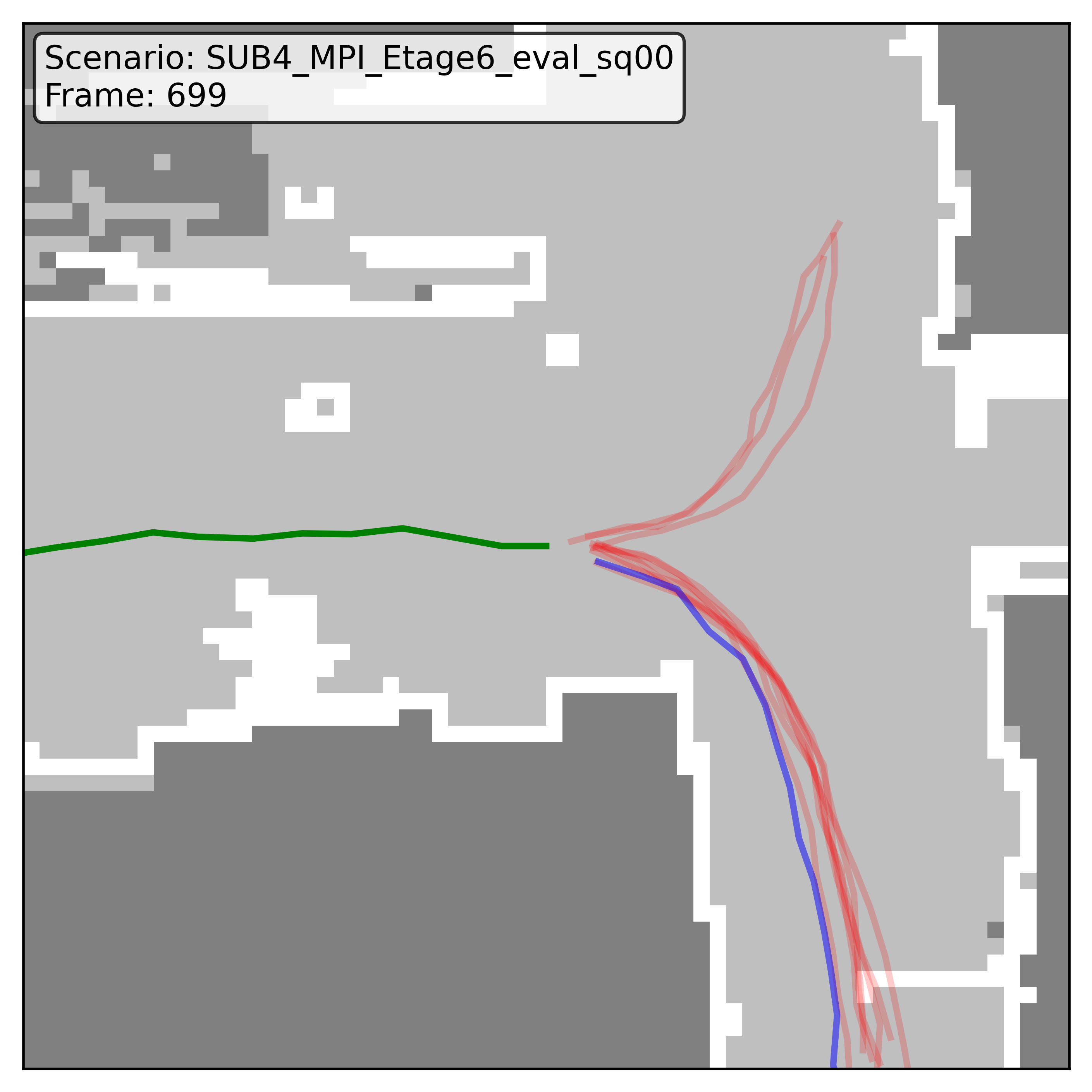
Correlation plot on GTA-IM — GTA-IM: quality vs truncation / SNR.

Correlation plot on HPS — HPS: quality vs truncation / SNR.

Qualitative examples

Below are example predictions from both datasets. You can see the behavior is stable as long as we do not truncate too aggressively.

GTA qualitative prediction — GTA-IM example (Dif-TR 0.50).

HPS qualitative prediction — HPS example (Dif-TR 0.50).

Final message

We can make diffusion faster in sequential prediction by reusing what we already know from the previous frame.

The method is simple, theory-backed, and practical for real-time robotics settings.